

This is based on a talk I gave at DeFi.WTF in Osaka around Devcon 5. WTF published a video and transcript here.
One way to think about “value” is through the lens of costs. The basic principle is that markets allocate value along the lines of costs as they trend to equilibrium. So we can estimate the overall behavior of future value by studying its associated cost structure. To establish this logic we’ll review some fundamental principles of economics (based on equilibrium and MB=MC) and piece apart what we mean by “costs”. Then we’ll apply this insight to reason about the nature of value capture and investment returns in crypto.
First is the model for equilibrium found in most (all?) Econ 101 textbooks:
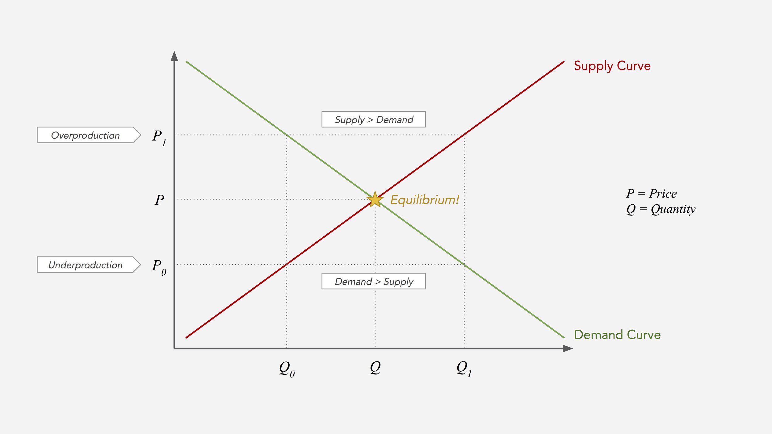
P and Q represent price and production levels. P*Q represents total economic value. The curves represent how much Supply and Demand is available at different price and quantity levels. Their actual shapes and slopes vary by infinite factors. But in general, the supply curve trends up because higher price levels attract more Supply and the demand curve trends down because lower price levels attract Demand.
Markets are in equilibrium when supply matches demand. Whenever prices rise above this point, there is more supply (Q1) than there is demand (Q0). The supply side has over-produced and will have to lower prices to meet demand. When prices dip below equilibrium, we’ve underproduced (Q0) when there is excess demand (Q1), driving prices up.
In the short-run, the economy is rarely in equilibrium: markets fluctuate from underproduction to overproduction, and from underpricing to overpricing at a regular cadence due to many factors. But they trend towards equilibrium in the long run because the alternatives are unsustainable and weak links (e.g. failing businesses) disappear over time.
MB=MC
One level down, at the margin, the principle of allocative efficiency establishes that at equilibrium, marginal benefit (price) equals marginal cost (MB=MC):
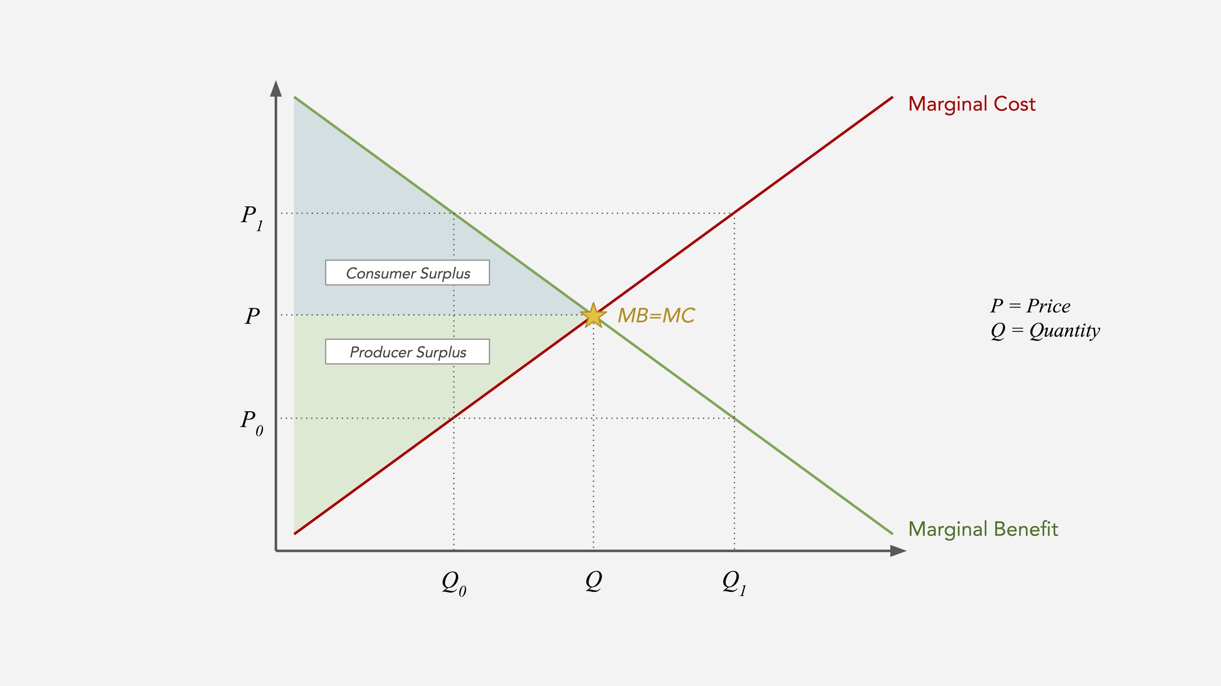
The marginal benefit curve shows what consumers are willing to pay at different supply levels; in essence, its “value” as measured by price. The marginal cost curve describes the *economic* costs of production for each unit. Again, the shapes of these curves vary widely from case to case. But in general MB trends down because the more abundant a good the less valuable it is in the market (see the law of diminishing marginal utility), while MC trends up because costs tend to go up as production scales (see the law of diminishing returns).
MB=MC is the optimal price point because it’s when the producer recovers all the costs of production (including any margins, more on that below) and consumers pay the lowest possible price. It’s also when both consumer and producer surplus (i.e. the total value to each side of the transaction) are maximized. For the consumer, it’s the area below the marginal benefit curve and above the price (the delta between the price paid and the value received), and for the producer, it’s the one above the marginal cost curve and below the price (the delta between price and cost). A different to explore this idea is by studying Gossen’s second law.
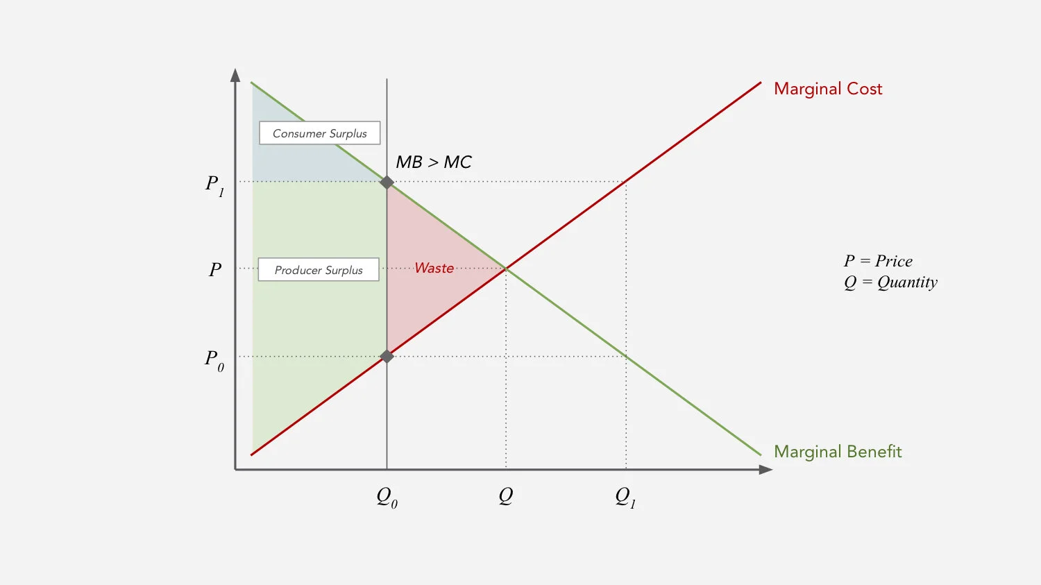
Whenever marginal benefit does not equal marginal cost, there’s some inefficiency. For example, MB > MC means there’s less of a good being produced (Q0) than is optimal (Q). This advantages the producer over the consumer because the price (P1), as determined by MB, is above the cost of production (P0) as determined by MC. This market failure shows up as economic “waste” in the form of unmet demand:
MB<MC does the opposite. Consumers benefit at the expense of producers when market price sits below the cost of production, and waste shows up in the form of losses to the producer:

Policy is a common cause of market failure. For example, MB>MC can be induced by artificial scarcity rules or even quantitative easing, and MB<MC by discrete price limits or subsidies. But of course other kinds of market failures, such as monopolies, can cause similar imbalances. For example, Big Web data monopolies can be seen as inducing MB>MC by constraining the supply of Information by instituting data silos.
Economic Costs
MB=MC suggests things are worth, or at least priced at what they cost to make or buy. Actually, it’s more useful to think of it as what it costs to replace. For example, the replacement cost of a widely available commodity is much lower than that of a famous work by a deceased artist. Interestingly, this way of thinking about the value of things is commonly used by tax collectors and insurance appraisers.
Anyways, if something is priced below its cost, it’s unprofitable to the seller. If they’re priced well above costs, there’s an inefficiency the market will seek to correct. These ideas can be confusing in a business context where companies have profit margins, for instance. But from an economics perspective, “costs” include all manner of things, such as the cost of capital, risk, competition, and so on. MB=MC makes sense when you consider all economic costs and externalities, known and unknown, not just the “accounting” costs.
For example, venture capital is “expensive capital” because it comes with high return requirements to compensate for the risk. This means the risk-adjusted cost of capital for a venture-funded business is very high. So a tech startup, for example, may show 80% gross margins in an accounting sense, but from an economics perspective, we think of those as the cost of expensive capital. A consistent, low-risk business in a stable environment would have a lower cost of capital and therefore command lesser margins to pay it back.
TV=TC
From MB=MC we can derive a final principle, that Total Value equals Total Cost (TV=TC). Total Value (gross) is synonymous with Total Benefit, which is the sum of all marginal benefits (as measured by Price). Total Costs is the sum of all marginal costs. So if MB=MC, it follows that at equilibrium TV=TC.How To Think About Value
TV=TC describes a direct relationship between costs and value. And while it relies on a number of “equilibrium” assumptions, we can use it to establish a general logic for thinking about value. Long-run, markets allocate value along the lines of costs. So to find value, look for costs. This insight is useful because observing costs is more practical than speculating on future profits.There’s a lot of debate and modern criticisms around the accuracy of these basic principles – mostly out of a search for precision in economic modeling. But the value of economic models is to help us see more by looking at less. Here, we’re not looking to establish a specific formula for valuing something so much as a general logic for thinking about how value is created, determined and distributed. These models help us think about value in a more fundamental sense, which can help us reason about other things like investment returns.
On that topic, there’s another nuance worth stressing: value capture does not equal investment returns. We can use this logic to predict overall distribution or “capture” of value across an economy, a market, a value chain or even within a firm. But value capture is more of a TAM input, related but independent of returns. Returns are a function of cost basis, growth rate, and ownership concentration among other things.
You can experience low returns in markets with high value “captured,” but where capital requirements are high, the risk is low and growth is nominal. Utilities, for example, capture a lot of value “on balance sheet” in the form of expensive infrastructure and other assets, but are otherwise thin-margin, low-growth businesses that serve more to store value at scale than grow it. On the opposite end, you can find high returns in new markets with less value captured, in opportunities with low capital requirements (so you can own a larger piece for the money), high risk, but high growth potential as is the case with the venture-startup complex.
On Value in Crypto
To end with some crypto points, are some quick insights to be expanded in later work:
Cryptonetworks, as markets, will seek equilibrium or collapse. So their economic models, as policy, must be conducive to equilibrium. When designing cryptoeconomic models, allocate value along the lines of costs. Borrowing the cryptoeconomic circle, it means considering the cost of production for the supply side, the cost of capital for investors, and the value to users. Advantaging one group over the other, for example by over-allocating value to investors when most of the costs are expected to be taken by supply-siders, can be destructive.
A good example of value allocation done right is Decred, a Bitcoin alternative where block reward inflation is distributed 60% to proof-of-work miners (who bear the highest costs), 30% to the proof-of-stake voters (who bear the cost of capital from buying and staking DCR), and 10% to the Decred treasury to cover the cost of long-term network development.
The basis of value for a network token lies in its costs of production and capital. If a token is created through mining or other type of work, part of its intrinsic value will be the costs of production for the supply side. E.g. if you’ve invested $1 million into a mining operation that will produce 10,000 tokens, $100/token becomes your preferred minimum price and you’ll be unlikely to sell below that point. But when it comes to economic costs, you also have to consider things like the cost of capital for its investors. For example, if you invested $1 million into the same 10,000 tokens with 3x return expectation, your minimum price becomes $300/token. All of these things happen at the margin, but the sum of the parts take us back to TV=TC (again, considering economic costs beyond accounting costs). Now, in the short run, we of course see a lot of deviation from equilibrium especially in crypto where the market is quite immature. For example, the overproduction of smart contract platforms means the market will demand lower pricing to find equilibrium, something we’re already seeing. That is good and bad depending on where you sit.
Protocols are higher-cost than applications. Protocols provide scale and require more investment, so they demand more of the value to maintain equilibrium. Applications command less value because they take on less of the costs. For proper scale, always consider the value of an individual application in relation to the combined value of all the protocols they use.
Returns can move around as markets develop. Today there are outsized returns available at the protocol layer as it remains high-risk. In the long run, they may scale to store trillions in value but with flat growth. Most of the value may remain “captured” at that layer as returns shift to the application layer where there is more competition. But we’re far from that equilibrium.
Distribute costs to distribute value. We explored this idea in an article comparing web and crypto service models. A deeper understanding of the “economic physics” of costs and value is key if our goal is to design systems that distribute value more broadly. Long-term, markets will naturally allocate value to those who bear the costs and risks.